fearec
fisher eigen analyser for recombination
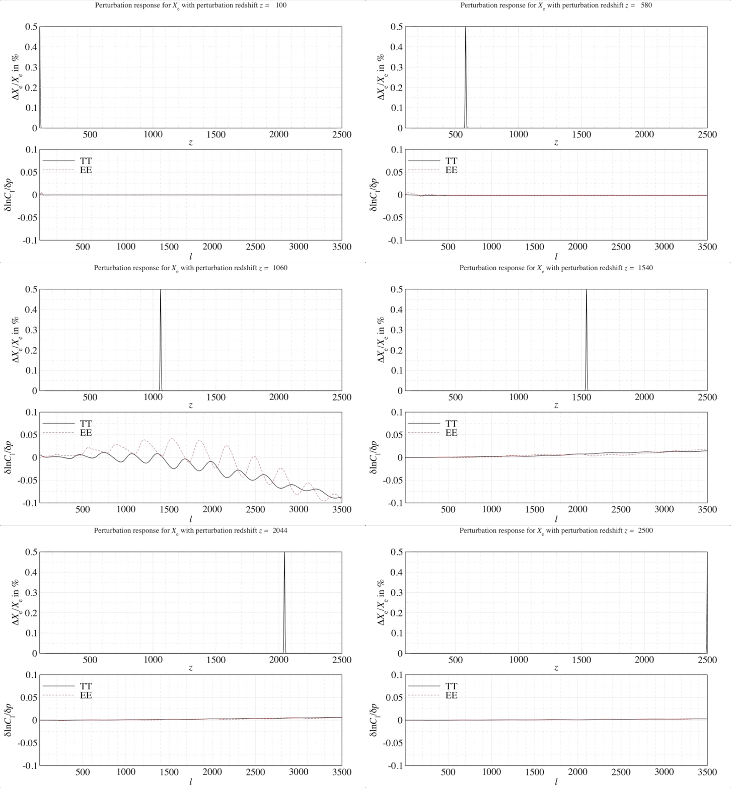
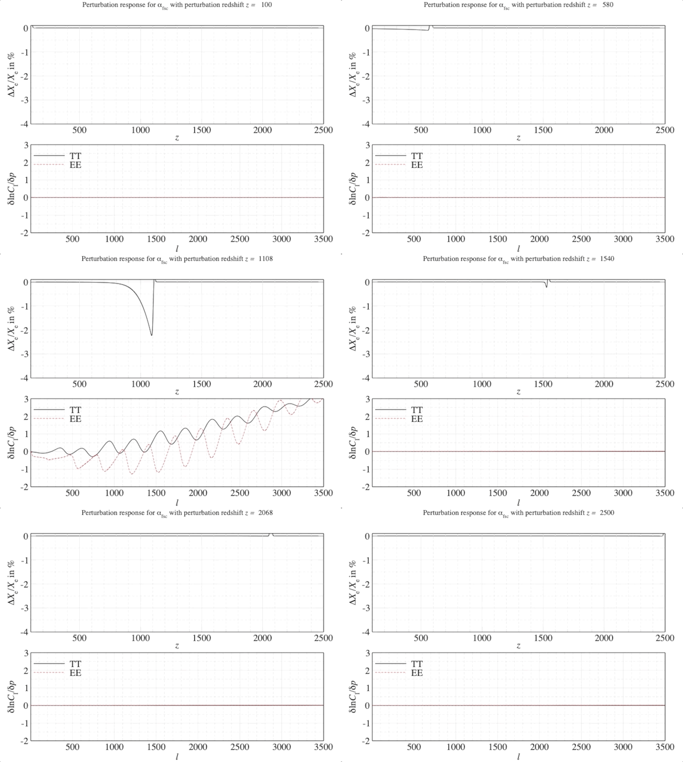
Introducing FEARec or FEARec++ (Fisher Eigen Analyser for Recombination) which can be used to solve a functional principal component analysis for problems that are closed at finite limits for generic parameter changes. In this case, the variation impacts the free-electron fraction \(X_{\rm e}\) which changes how many electrons in the early Universe are ionised from their nuclei due to the hot background of photons known now as the cosmic microwave background (CMB).
The smooth, time (redshift) dependent variations for this fraction are then cast onto the anisotropies of the CMB. These anisotropies are tiny fluctuations in temperature across the sky which tell us how the constituents of the Universe were distributed at very early times. By reverse engineering the largest changes, using a small bit of linear algebra, we can reconfigure these functional variations in a parameter (here \(X_{\rm e}\)).


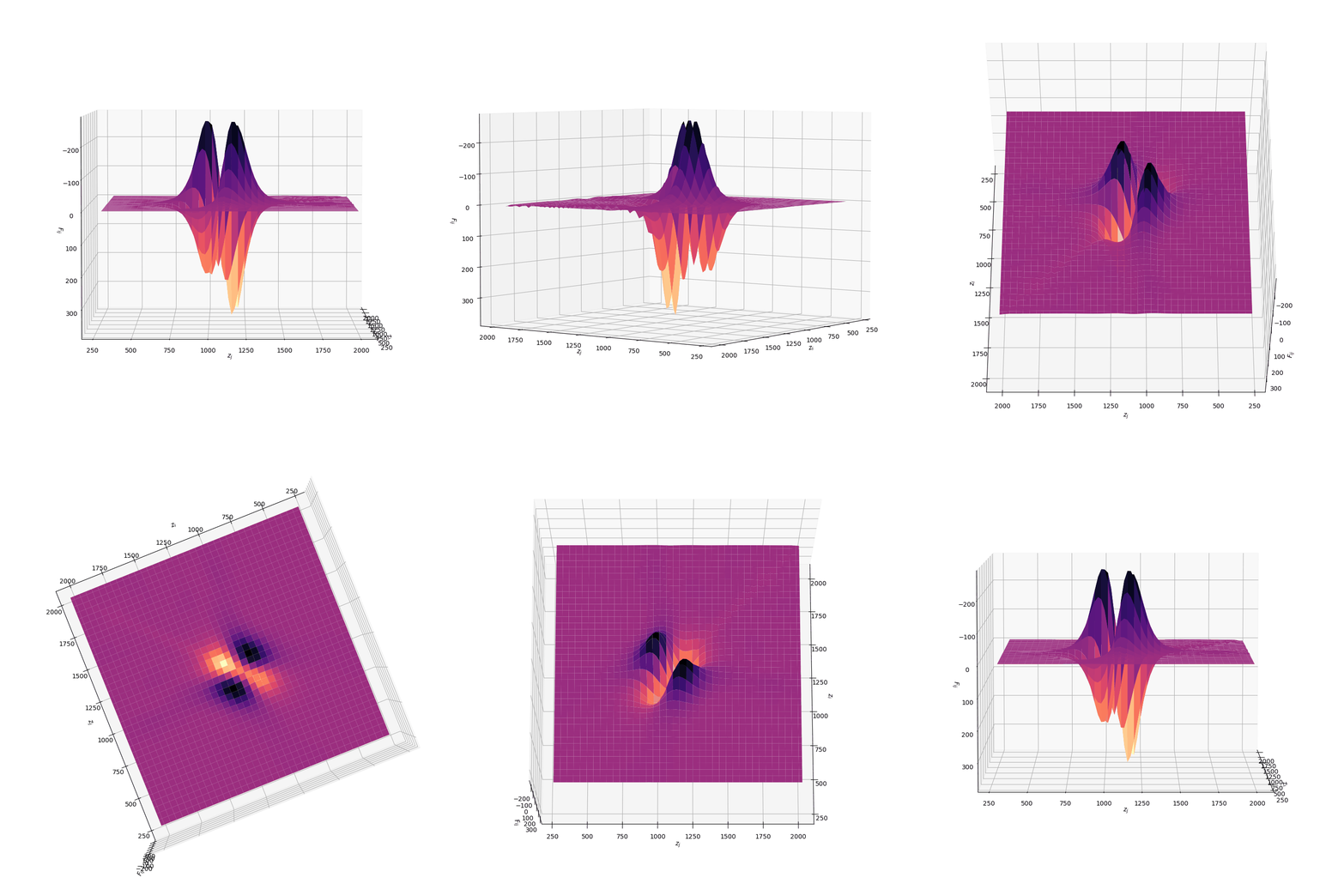
We can weight the responses in the CMB spectra by the relative signal-to-noise in a given observable channel (in this case, the multipoles \(\ell\) of the CMB anisotropies). Once we have seen the response of the CMB spectra, this can be quantified by a mathematical object known as a Fisher matrix. The weighted responses are known as Fisher matrix elements \(F_{ij}\) and once this has been constructed we can transform this matrix into the leading order dimensions with the highest responses (or highest SNR).

Code implementation
FEARec uses several important aspects of programming to complete the analysis but first and foremost, it is developed in C++ to optimise for object oriented programming. In this framework, I have also developed a Makefile for console usage of the routines (once they have been further optimised for better UX). Specifically, the components of the responses in the CMB power spectra, the Fisher matrix itself and the likelihood data management project (for directly taking likelihood samples) are all held in their own classes. These classes then store as standard and then utilise the Eigen collection of headers which make linear algebra much simpler. This includes eigen-solver classes, An example of this is below where we generate the eigenmodes for the Fisher analysis:
void fisher::get_modes(Eigen::VectorXd &xarr, Eigen::MatrixXd &eigenmodes, Eigen::VectorXd &eigenvalues, int truncate) {
    Eigen::SelfAdjointEigenSolver<Eigen::MatrixXd> solver(this->fisher_matrix);
    eigenmodes = solver.eigenvectors().rightCols(truncate);
    eigenvalues = solver.eigenvalues().tail(truncate);

    xarr=Eigen::VectorXd(eigenmodes.rows());
    for (int k = 0; k < eigenmodes.rows(); k++)  {
        int kk=utils::mult_factor*k;
        xarr(k) = utils::counter_to_redshift(kk);
    }
    // When we interpolate on a grid lower resolution than 0.5,
    // modes start to become destabilised within the Boltzmann code
    if (utils::mode_dz > .5) {
      utils::print_warning("get_modes",
                           "Low resolution splines are difficult to constrain!");
    }
    interp_function(xarr,eigenmodes,eigenvalues,utils::mode_dz);

    for (int i=0; i < eigenvalues.size(); i++) {
      if (utils::eigenvalue_errors) eigenvalues(i) = sqrt(1/eigenvalues(i));
    }
    return;
}
Here we have interpolation routines that refine the eigenmodes and print the errors according to the Kramer-Rao definition.
For more details on the FEARec project please visit GitHub to see the latest updates on the project.